class: center, middle, inverse, title-slide # Visualization - Aesthetic Mapping - Titanic --- class: inverse, middle, center --- # A visualization: -- - is a geometry object (a geom) -- - whose aesthetics -- - represents variables -- - from a data set --- # Aesthetics mean -- - “something you can see”. -- Examples include: - position (i.e., on the x and y axes) - color (“outside” color) - fill (“inside” color) - shape (of points) - size --- # Aesthetics Mapping -- - map -- - variables -- - to aesthetics --- class: inverse, middle, center # Examples --- ```r library(tidyverse) library(ggplot2) df <- read_csv('https://bryantstats.github.io/math421/data/titanic.csv') df <- df %>% mutate(Survived = as.character(Survived), Pclass = as.character(Pclass)) ``` --- ```r df %>% ggplot()+ geom_density(mapping = aes(x = Age, color=Survived)) ``` 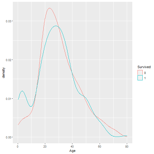<!-- --> --- # Aesthetic of a geom - A geom has its list of own aesthetics - Use `?geom_point()` to check for the list of `geom_point` - Some aesthetics are required, some are not --- class: inverse, middle, center # Common Visualization Practices --- # One Continuous Variable - Density: `geom_density` - Histogram: `geom_histogram` - Boxplot: `geom_boxplot` --- **One Continuous Variable: Density** ```r df %>% ggplot()+ geom_density(mapping = aes(x = Age)) ``` 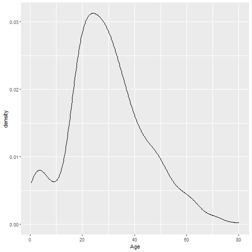<!-- --> --- **One Continuous Variable: Histogram** ```r df %>% ggplot()+ geom_histogram(mapping = aes(x = Age)) ``` 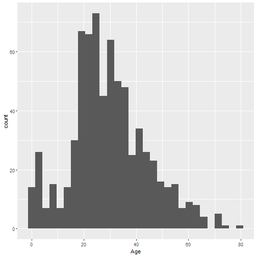<!-- --> --- **One Categorical Variable: Bar chart** ```r df %>% ggplot()+ geom_bar(mapping = aes(x = Survived)) ``` 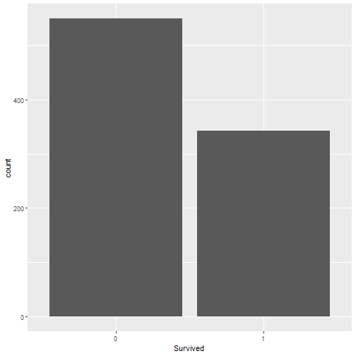<!-- --> --- # Two Continuous Variables - Scatter Plot: `geom_point` - Line Plot: `geom_line` - Smooth Plot: `geom_smooth` --- **Two numeric: Scatter Plot: `geom_point`** ```r df %>% ggplot()+geom_point(aes(x=Age, y=Fare)) ``` 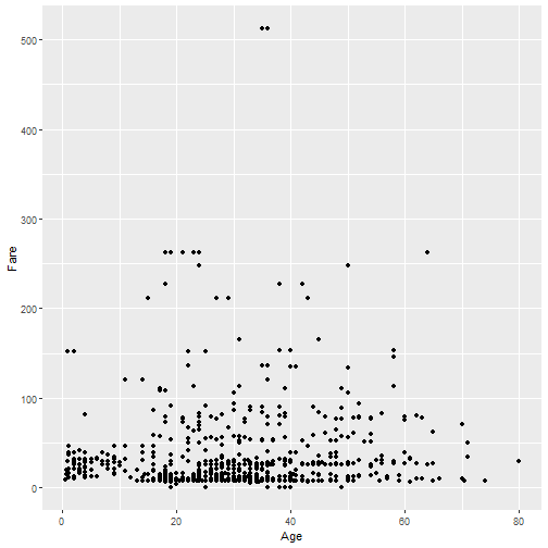<!-- --> --- **Two numeric: Line Plot: `geom_line`** ```r df %>% ggplot()+geom_line(aes(x=Age, y=Fare)) ``` 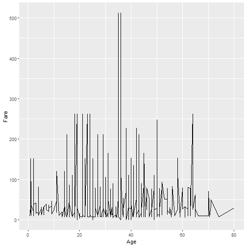<!-- --> --- **Two numeric: Smooth Plot: `geom_smooth`** ```r df %>% ggplot()+geom_smooth(aes(x=Age, y=Fare)) ``` 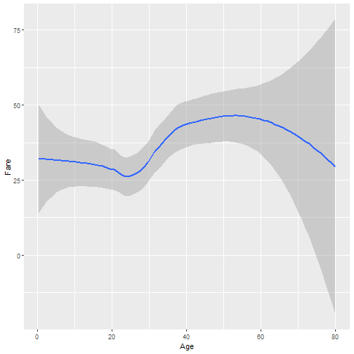<!-- --> --- **Two numeric: geom_point + geom_smooth** ```r df %>% ggplot() + geom_point(aes(x=Age, y=Fare))+ geom_smooth(aes(x=Age, y=Fare)) ``` 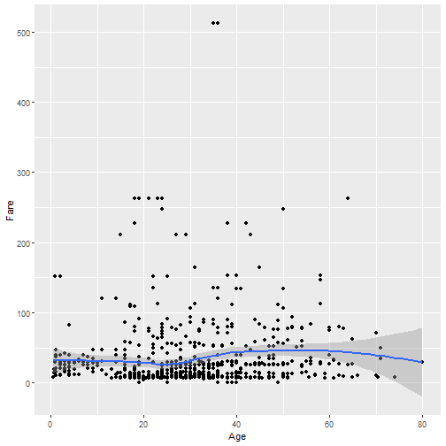<!-- --> --- # One Continuous Variable + One Categorical Variable - Density - BoxPlot --- **One Continuous + One Categorical: Density** ```r df %>% ggplot()+ geom_density(mapping = aes(x = Age, color = Survived)) ``` <!-- --> --- **One Continuous + One Categorical: Boxplot** ```r df %>% ggplot()+ geom_boxplot(mapping = aes(x = Age, y = Survived)) ``` 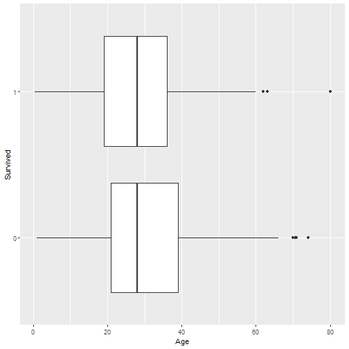<!-- --> --- # Two categorical variables - Barplot --- **Two categorical variables: Barplot** ```r df %>% ggplot()+ geom_bar(mapping=aes(x=Sex, fill=Survived), position = 'fill') ``` 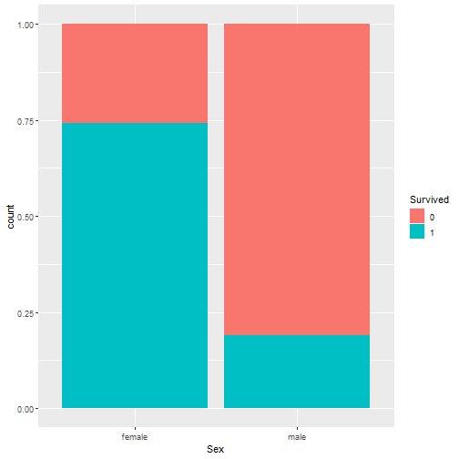<!-- --> --- ** Three variables** ```r df %>% ggplot() + geom_point(aes(x=Age, y=Fare, color = Survived)) ``` 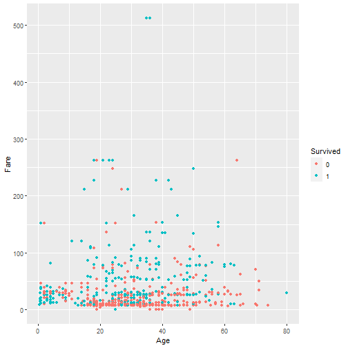<!-- --> --- # More - [ggplot cheat sheet](https://raw.githubusercontent.com/rstudio/cheatsheets/main/data-visualization.pdf)