Writing Functions

class: center, middle, inverse, title-slide

# <img src="figures/Thanksgiving-Day.jpg" /> Writing Functions - Basic
### <font size="5"> Son Nguyen </font>

---

<style>

.remark-slide-content {
  background-color: #FFFFFF;
  border-top: 80px solid #F9C389;
  font-size: 14px;
  font-weight: 300;
  line-height: 1.5;
  padding: 1em 1em 1em 1em
}

.inverse {
  background-color: #696767;
  border-top: 80px solid #696767;
  text-shadow: none;
  background-image: url(https://github.com/goodekat/presentations/blob/master/2019-isugg-gganimate-spooky/figures/spider.png?raw=true);
	background-position: 50% 75%;
  background-size: 150px;
}

.your-turn{
  background-color: #8C7E95;
  border-top: 80px solid #F9C389;
  text-shadow: none;
  background-image: url(https://github.com/goodekat/presentations/blob/master/2019-isugg-gganimate-spooky/figures/spider.png?raw=true);
	background-position: 95% 90%;
  background-size: 75px;
}

.title-slide {
  background-color: #F9C389;
  border-top: 80px solid #F9C389;
  background-image: none;
}

.title-slide > h1  {
  color: #111111;
  font-size: 40px;
  text-shadow: none;
  font-weight: 400;
  text-align: left;
  margin-left: 15px;
  padding-top: 80px;
}
.title-slide > h2  {
  margin-top: -25px;
  padding-bottom: -20px;
  color: #111111;
  text-shadow: none;
  font-weight: 300;
  font-size: 35px;
  text-align: left;
  margin-left: 15px;
}
.title-slide > h3  {
  color: #111111;
  text-shadow: none;
  font-weight: 300;
  font-size: 25px;
  text-align: left;
  margin-left: 15px;
  margin-bottom: -30px;
}

</style>

.pull-left {
  color: #777;
  width: 40%;
  height: 92%;
  float: left;
}
.pull-right {
  width: 59%;
  float: right;
  padding-left: 1%;
}

</style>

# Motivation

.pull-left[

- Plot words frequency of a text data

]

.pull-right[

]

---
# Motivation

.pull-left[

- Plot words frequency of a text data

- Sample Codes

]

.pull-right[

```r
df <- read_csv('../data/netflix_titles.csv')
df %>% 
  unnest_tokens(input = description, output = word) %>% 
  anti_join(get_stopwords()) %>% 
  count(word, sort = TRUE) %>% 
  head(5) %>% 
  ggplot(aes(x = n, y = reorder(word, n))) +
  geom_col() + theme(axis.text.y = element_text(size = 40))+ 
  labs(y = '', x = 'Frequency')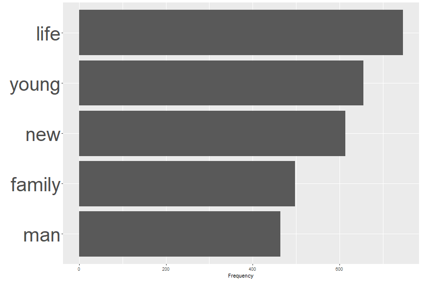
```

![](Figs/unnamed-chunk-3-1.png)

]

---
# Motivation

.pull-left[

- Plot words frequency of a text data

- Sample Codes

- Copy and Paste to another data

]

.pull-right[

```r
df <- read_tsv('../data/user_reviews.tsv')
df %>% 
  unnest_tokens(input = text, output = word) %>% 
  anti_join(get_stopwords()) %>% 
  count(word, sort = TRUE) %>% 
  head(5) %>% 
  ggplot(aes(x = n, y = reorder(word, n))) +
  geom_col() + theme(axis.text.y = element_text(size = 40))+ 
  labs(y = '', x = 'Frequency')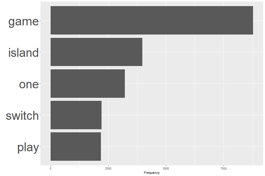
```

![](Figs/unnamed-chunk-4-1.png)

]

---
# Motivation

.pull-left[

- Plot words frequency of a text data

- Sample Codes

- Copy and Paste to another data

- Keep Copy and Paste

]

.pull-right[

```r
df <- read_csv('../data/spam_message.csv')
df %>% 
  unnest_tokens(input = Message, output = word) %>% 
  anti_join(get_stopwords()) %>% 
  count(word, sort = TRUE) %>% 
  head(5) %>% 
  ggplot(aes(x = n, y = reorder(word, n))) +
  geom_col() + theme(axis.text.y = element_text(size = 40))+
  labs(y = '', x = 'Frequency')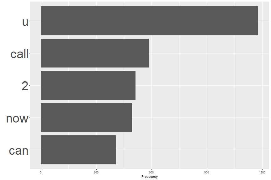
```

![](Figs/unnamed-chunk-5-1.png)

]

---
# Motivation

.pull-left[

- Plot words frequency of a text data

- Sample Codes

- Copy and Paste to another data

- Keep Copy and Paste

]

.pull-right[

```r
df <- read_csv('../data/netflix_titles.csv')
df %>% 
  unnest_tokens(input = director, output = word) %>% 
  anti_join(get_stopwords()) %>% 
  count(word, sort = TRUE) %>% 
  head(5) %>% 
  ggplot(aes(x = n, y = reorder(word, n))) +
  geom_col() + theme(axis.text.y = element_text(size = 40))+ 
  labs(y = '', x = 'Frequency')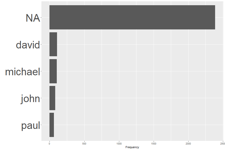
```

![](Figs/unnamed-chunk-6-1.png)

]

---
# Motivation

.pull-left[

- Plot words frequency of a text data

- Sample Codes

- Copy and Paste to another data

- Keep Copy and Paste

]

.pull-right[

```r
df <- read_csv('../data/netflix_titles.csv')
df %>% 
  unnest_tokens(input = cast, output = word) %>% 
  anti_join(get_stopwords()) %>% 
  count(word, sort = TRUE) %>% 
  head(5) %>% 
  ggplot(aes(x = n, y = reorder(word, n))) +
  geom_col() + theme(axis.text.y = element_text(size = 40))+ 
  labs(y = '', x = 'Frequency')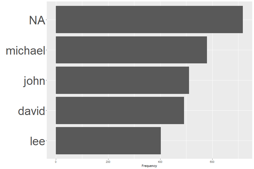
```

![](Figs/unnamed-chunk-7-1.png)

]

---
# Motivation

.pull-left[

- Copy and Paste a lot = Write a function

]

.pull-right[

]

---
# Motivation

.pull-left[

- Copy and Paste a lot = Write a function

- Write thas has

- Input: 
  
      - a data frame that has a text column 
    
      - the name of the text column in the data
  
  - Output: the plot of words frequency of the text column

]

.pull-right[

]

---
# Motivation

.pull-left[

- Copy and Paste a lot = Write a function

- Write thas has

- Input: 
  
      - a data frame that has a text column 
    
      - the name of the text column in the data
  
  - Output: the plot of words frequency of the text column

]

.pull-right[

```r
word_frequency <- function(text_df, text_col) {
  library(tidyverse)
  library(tidytext)
  text_df %>% 
  unnest_tokens(input = text_col, output = word) %>% 
  anti_join(get_stopwords()) %>% 
  count(word, sort = TRUE) %>% 
  head(5) %>% 
  ggplot(aes(x = n, y = reorder(word, n))) +
  geom_col() + theme(axis.text.y = element_text(size = 40))+ 
  labs(y = '', x = 'Frequency')
}
```

]

---
# Motivation

.pull-left[

- just call the function to do the task

]

.pull-right[

```r
df <- read_csv('../data/netflix_titles.csv')
word_frequency(text_df = df, text_col = 'description')
```

![](Figs/unnamed-chunk-9-1.png)

]

---
# Motivation

.pull-left[

- just call the function to do the task

]

.pull-right[

```r
df <- read_tsv('../data/user_reviews.tsv')
word_frequency(text_df = df, text_col = 'text')
```

![](Figs/unnamed-chunk-10-1.png)

]

---
# Motivation

.pull-left[

- just call the function to do the task

]

.pull-right[

```r
df <- read_csv('../data/spam_message.csv')
word_frequency(text_df = df, text_col = 'Message')
```

![](Figs/unnamed-chunk-11-1.png)

]

---
# Task 1

.pull-left[

- Solve and print out the solutions

`$$x^2+3x+2=0$$`

]

.pull-right[

]

---
# Task 1

.pull-left[

- Solve and print out the solutions

`$$x^2+3x+2=0$$`

]

.pull-right[

- Use the quadratic formula.

```r
a = 1
b = 3
c = 2

x1 <- (-b - sqrt(b^2 - 4*a*c))/(2*a)

x2 <- (-b + sqrt(b^2 - 4*a*c))/(2*a)

print(paste0('The solution are ', x1, ' and ', x2, '!'))
```

```
## [1] "The solution are -2 and -1!"
```

]

---
# Task 2

.pull-left[

- Solve and print out the solutions

`$$x^2 - 8x + 12 = 0$$`

`$$x^2 - 4x + 3 = 0$$`

`$$x^2 + 5x + 6 = 0$$`
]

.pull-right[

]

---
# Task 2

.pull-left[

- Solve and print out the solutions

`$$x^2 - 8x + 12 = 0$$`

`$$x^2 - 4x + 3 = 0$$`

`$$x^2 + 5x + 6 = 0$$`
]

- Approach 1: Copy/Paste/Edit

.pull-right[

]

---
# Task 2

.pull-left[

- Solve and print out the solutions

`$$x^2 - 8x + 12 = 0$$`

`$$x^2 - 4x + 3 = 0$$`

`$$x^2 + 5x + 6 = 0$$`
]

- Approach 1: Copy/Paste/Edit

.pull-right[

```r
a = 1
b = -8
c = 12

x1 <- (-b - sqrt(b^2 - 4*a*c))/(2*a)

x2 <- (-b + sqrt(b^2 - 4*a*c))/(2*a)

print(paste0('The solution are ', x1, ' and ', x2, '!'))
```

```
## [1] "The solution are 2 and 6!"
```

]

---
# Task 2

.pull-left[

- Solve and print out the solutions

`$$x^2 - 8x + 12 = 0$$`

`$$x^2 - 4x + 3 = 0$$`

`$$x^2 + 5x + 6 = 0$$`
]

- Approach 1: Copy/Paste/Edit

.pull-right[

```r
a = 1
b = -4
c = 3

x1 <- (-b - sqrt(b^2 - 4*a*c))/(2*a)

x2 <- (-b + sqrt(b^2 - 4*a*c))/(2*a)

print(paste0('The solution are ', x1, ' and ', x2, '!'))
```

```
## [1] "The solution are 1 and 3!"
```

]

---
# Task 2

.pull-left[

- Solve and print out the solutions

`$$x^2 - 8x + 12 = 0$$`

`$$x^2 - 4x + 3 = 0$$`

`$$x^2 + 5x + 6 = 0$$`
]

- Approach 1: Copy/Paste/Edit

.pull-right[

```r
a = 1
b = 5
c = 6

x1 <- (-b - sqrt(b^2 - 4*a*c))/(2*a)

x2 <- (-b + sqrt(b^2 - 4*a*c))/(2*a)

print(paste0('The solution are ', x1, ' and ', x2, '!'))
```

```
## [1] "The solution are -3 and -2!"
```

]

---
# Task 2

.pull-left[

- Solve and print out the solutions

`$$x^2 - 8x + 12 = 0$$`

`$$x^2 - 4x + 3 = 0$$`

`$$x^2 + 5x + 6 = 0$$`
]

- Approach 2: Write a function

.pull-right[
]

---
# Task 2

.pull-left[

- Solve and print out the solutions

`$$x^2 - 8x + 12 = 0$$`

`$$x^2 - 4x + 3 = 0$$`

`$$x^2 + 5x + 6 = 0$$`
]

- Approach 2: Write a function

.pull-right[

```r
qdr <- function(a, b, c)
{
  x1 <- (-b - sqrt(b^2 - 4*a*c))/(2*a)

x2 <- (-b + sqrt(b^2 - 4*a*c))/(2*a)

print(paste0('The solution are ', x1, ' and ', x2, '!'))
}
```
]

---
# Task 2

.pull-left[

- Solve and print out the solutions

`$$x^2 - 8x + 12 = 0$$`

`$$x^2 - 4x + 3 = 0$$`

`$$x^2 + 5x + 6 = 0$$`
]

- Approach 2: Write a function

.pull-right[

```r
qdr <- function(a, b, c)
{
  x1 <- (-b - sqrt(b^2 - 4*a*c))/(2*a)

x2 <- (-b + sqrt(b^2 - 4*a*c))/(2*a)

print(paste0('The solution are ', x1, ' and ', x2, '!'))
}
```

```r
qdr(a = 1, b = -8, c = 12)
```

```
## [1] "The solution are 2 and 6!"
```

]

---
# Task 2

.pull-left[

- Solve and print out the solutions

`$$x^2 - 8x + 12 = 0$$`

`$$x^2 - 4x + 3 = 0$$`

`$$x^2 + 5x + 6 = 0$$`
]

- Approach 2: Write a function

.pull-right[

```r
qdr <- function(a, b, c)
{
  x1 <- (-b - sqrt(b^2 - 4*a*c))/(2*a)

x2 <- (-b + sqrt(b^2 - 4*a*c))/(2*a)

print(paste0('The solution are ', x1, ' and ', x2, '!'))
}
```

```r
qdr(a = 1, b = -8, c = 12)
```

```
## [1] "The solution are 2 and 6!"
```

```r
qdr(a = 1, b = -4, c = 3)
```

```
## [1] "The solution are 1 and 3!"
```

]

---
# Task 2

.pull-left[

- Solve and print out the solutions

`$$x^2 - 8x + 12 = 0$$`

`$$x^2 - 4x + 3 = 0$$`

`$$x^2 + 5x + 6 = 0$$`
]

- Approach 2: Write a function

.pull-right[

```r
qdr <- function(a, b, c)
{
  x1 <- (-b - sqrt(b^2 - 4*a*c))/(2*a)

x2 <- (-b + sqrt(b^2 - 4*a*c))/(2*a)

print(paste0('The solution are ', x1, ' and ', x2, '!'))
}
```

```r
qdr(a = 1, b = -8, c = 12)
```

```
## [1] "The solution are 2 and 6!"
```

```r
qdr(a = 1, b = -4, c = 3)
```

```
## [1] "The solution are 1 and 3!"
```

```r
qdr(a = 1, b = 5, c = 6)
```

```
## [1] "The solution are -3 and -2!"
```

]

---
# Easy to fix an error

.pull-left[

- Notice there is a typo!

]

.pull-right[]

---
# Easy to fix an error

.pull-left[

- Notice there is a typo!

- Just need to edit the function
]

.pull-right[]

---
# Easy to fix an error

.pull-left[

- Notice there is a typo!

- Just need to edit the function
]

.pull-right[

```r
qdr <- function(a, b, c)
{
  x1 <- (-b - sqrt(b^2 - 4*a*c))/(2*a)

x2 <- (-b + sqrt(b^2 - 4*a*c))/(2*a)

print(paste0('The solutions are ', x1, ' and ', x2, '!'))
}
```
]

---
# Easy to fix an error

.pull-left[

- Notice there is a typo!

- Just need to edit the function
]

.pull-right[

```r
qdr <- function(a, b, c)
{
  x1 <- (-b - sqrt(b^2 - 4*a*c))/(2*a)

x2 <- (-b + sqrt(b^2 - 4*a*c))/(2*a)

print(paste0('The solutions are ', x1, ' and ', x2, '!'))
}
```

```r
qdr(1, -8, 12)
```

```
## [1] "The solutions are 2 and 6!"
```

```r
qdr(1, -4, 3)
```

```
## [1] "The solutions are 1 and 3!"
```

```r
qdr(1, 5, 6)
```

```
## [1] "The solutions are -3 and -2!"
```

]

---
# When should you write a function?

- Whenever you do many copy/paste

---
# Default Arguments

.pull-left[

]

.pull-right[

```r
qdr <- function(a, b, c)
{
  x1 <- (-b - sqrt(b^2 - 4*a*c))/(2*a)

x2 <- (-b + sqrt(b^2 - 4*a*c))/(2*a)

print(paste0('The solutions are ', x1, ' and ', x2, '!'))
}
```

]

---
# Default Arguments

.pull-left[

- a, b, c are the arguments
]

.pull-right[

```r
qdr <- function(a, b, c)
{
  x1 <- (-b - sqrt(b^2 - 4*a*c))/(2*a)

x2 <- (-b + sqrt(b^2 - 4*a*c))/(2*a)

print(paste0('The solutions are ', x1, ' and ', x2, '!'))
}
```

]

---
# Default Arguments

.pull-left[

- a, b, c are the arguments
]

.pull-right[

```r
qdr <- function(a, b, c)
{
  x1 <- (-b - sqrt(b^2 - 4*a*c))/(2*a)

x2 <- (-b + sqrt(b^2 - 4*a*c))/(2*a)

print(paste0('The solutions are ', x1, ' and ', x2, '!'))
}
```

```r
qdr(a = 1, b = -3, c = 2)
```

```
## [1] "The solutions are 1 and 2!"
```
]

---
# Default Arguments

.pull-left[

- a, b, c are the arguments
]

.pull-right[

```r
qdr <- function(a, b, c)
{
  x1 <- (-b - sqrt(b^2 - 4*a*c))/(2*a)

x2 <- (-b + sqrt(b^2 - 4*a*c))/(2*a)

print(paste0('The solutions are ', x1, ' and ', x2, '!'))
}
```

```r
qdr(a = 1, b = -3, c = 2)
```

```
## [1] "The solutions are 1 and 2!"
```

```r
qdr(1, -3, 2)
```

```
## [1] "The solutions are 1 and 2!"
```

]

---
# Default Arguments

.pull-left[

- a, b, c are the arguments
]

.pull-right[

```r
qdr <- function(a, b, c)
{
  x1 <- (-b - sqrt(b^2 - 4*a*c))/(2*a)

x2 <- (-b + sqrt(b^2 - 4*a*c))/(2*a)

print(paste0('The solutions are ', x1, ' and ', x2, '!'))
}
```

```r
qdr(a = 1, b = -3, c = 2)
```

```
## [1] "The solutions are 1 and 2!"
```

```r
qdr(1, -3, 2)
```

```
## [1] "The solutions are 1 and 2!"
```

```r
qdr()
```

```
## Error in qdr(): argument "b" is missing, with no default
```

]

---
# Default Arguments

.pull-left[

- It's a good practice to set default arguments
]

.pull-right[

]

---
# Default Arguments

.pull-left[

- It's a good practice to set default arguments
]

.pull-right[

```r
qdr <- function(a = 1, b = 3, c = 2)
{
  x1 <- (-b - sqrt(b^2 - 4*a*c))/(2*a)

x2 <- (-b + sqrt(b^2 - 4*a*c))/(2*a)

print(paste0('The solutions are ', x1, ' and ', x2, '!'))
}
```
]

---
# Default Arguments

.pull-left[

- It's a good practice to set default arguments
]

.pull-right[

```r
qdr <- function(a = 1, b = 3, c = 2)
{
  x1 <- (-b - sqrt(b^2 - 4*a*c))/(2*a)

x2 <- (-b + sqrt(b^2 - 4*a*c))/(2*a)

print(paste0('The solutions are ', x1, ' and ', x2, '!'))
}
```

```r
qdr()
```

```
## [1] "The solutions are -2 and -1!"
```

]

---
# How to write a function

- Step 1: Decide the input

- Step 2: Know what you want for the output

---
# Example 1

.pull-left[

Write a function to convert a GPA from 4.0 scale to 10.0 scale and print out a statement: "You have `r` GPA" where `r` is the GPA in 10.0 scale.

- Input: a number, x

- Output:  "You have `r` GPA" where `r` is the GPA in 10.0 scale.

]

.pull-right[

]

---
# Example 1

.pull-left[

Write a function to convert a GPA from 4.0 scale to 10.0 scale and print out a statement: "You have `r` GPA" where `r` is the GPA in 10.0 scale.

- Input: a number, x

- Output:  "You have `r` GPA" where `r` is the GPA in 10.0 scale.

]

.pull-right[

- Write a function

```r
gpa <- function(x)
{
  r = (x/4)*10.0
  print(paste0('You have ', r, ' GPA in the 10.0 scale!'))
}
```

]

---
# Example 1

.pull-left[

Write a function to convert a GPA from 4.0 scale to 10.0 scale and print out a statement: "You have `r` GPA" where `r` is the GPA in 10.0 scale.

- Input: a number, x

- Output:  "You have `r` GPA" where `r` is the GPA in 10.0 scale.

]

.pull-right[

- Write a function

```r
gpa <- function(x)
{
  r = (x/4)*10.0
  print(paste0('You have ', r, ' GPA in the 10.0 scale!'))
}
```

- Test the function

```r
gpa(3.9)
```

```
## [1] "You have 9.75 GPA in the 10.0 scale!"
```

]

---
# Example 1

.pull-left[

Write a function to convert a GPA from 4.0 scale to 10.0 scale and print out a statement: "You have `r` GPA" where `r` is the GPA in 10.0 scale.

- Input: a number, x

- Output:  "You have `r` GPA" where `r` is the GPA in 10.0 scale.

]

.pull-right[

- Write a function

```r
gpa <- function(x)
{
  r = (x/4)*10.0
  print(paste0('You have ', r, ' GPA in the 10.0 scale!'))
}
```

- Test the function

```r
gpa(2)
```

```
## [1] "You have 5 GPA in the 10.0 scale!"
```

```r
gpa(4.0)
```

```
## [1] "You have 10 GPA in the 10.0 scale!"
```

]

---
# Example 2

.pull-left[

Write the following function.  Give an example to test your function.

- Input: a GPA, x

- Output:

- print: You are doing great! if x > 3.0, 
  - print: Keep working hard! otherwise

]

.pull-right[

]

---
# Example 2

.pull-left[

Write the following function.  Give an example to test your function.

- Input: a GPA, x

- Output:

- print: You are doing great! if x > 3.0, 
  - print: Keep working hard! otherwise

]

.pull-right[

- Write a function

```r
gpa2 <- function(x)
{
  if(x>3)
  {
    print('You are doing great!') 
  }
  
  else
  {
    print('Keep working hard!')
  }
}
```

]

---
# Example 2

.pull-left[

Write the following function.  Give an example to test your function.

- Input: a GPA, x

- Output:

- print: You are doing great! if x > 3.0, 
  - print: Keep working hard! otherwise

]

.pull-right[

- Write a function

```r
gpa2 <- function(x)
{
  if(x>3)
  {
    print('You are doing great!') 
  }
  
  else
  {
    print('Keep working hard!')
  }
}
```

- Test the function

```r
gpa2(2.9)
```

```
## [1] "Keep working hard!"
```

]

---
# Example 2

.pull-left[

Write the following function.  Give an example to test your function.

- Input: a GPA, x

- Output:

- print: You are doing great! if x > 3.0, 
  - print: Keep working hard! otherwise

]

.pull-right[

- Write a function

```r
gpa2 <- function(x)
{
  if(x>3)
  {
    print('You are doing great!') 
  }
  
  else
  {
    print('Keep working hard!')
  }
}
```

- Test the function

```r
gpa2(2.9)
```

```
## [1] "Keep working hard!"
```

```r
gpa2(3.5)
```

```
## [1] "You are doing great!"
```

]

---
# Example 3

.pull-left[

Write the following function.  Give an example to test your function.

- Input: a vector

- Output:

- if the vector is non-numeric, return the vector with missing values replaced by the mode (most frequent category).
  
  - if the vector is numeric, do nothing and return the same input vector

]

.pull-right[
]

---
# Example 3

.pull-left[

Write the following function.  Give an example to test your function.

- Input: a vector

- Output:

- if the vector is non-numeric, return the vector with missing values replaced by the mode (most frequent category).
  
  - if the vector is numeric, do nothing and return the same input vector

]

.pull-right[

- Write a function

```r
mode_impute <- function(x)
{
  if(!is.numeric(x))
  {
    # Find the mode of x
    mode_of_x <- names(sort(-table(x)))[1]
    
    # Replace the missing by the mode
    library(tidyr)
    x <- replace_na(x, mode_of_x) 
  }
return(x)    
}
```

]

---
# Example 3

.pull-left[

Write the following function.  Give an example to test your function.

- Input: a vector

- Output:

- if the vector is non-numeric, return the vector with missing values replaced by the mode (most frequent category).
  
  - if the vector is numeric, do nothing and return the same input vector

]

.pull-right[

- Write a function

- Test the function

```r
library(tidyverse)
df <- read_csv('titanic.csv')

x1 <- mode_impute(df$Embarked)
sum(is.na(x1))
```

```
## [1] 0
```

]

---
# Example 3

.pull-left[

Write the following function.  Give an example to test your function.

- Input: a vector

- Output:

- if the vector is non-numeric, return the vector with missing values replaced by the mode (most frequent category).
  
  - if the vector is numeric, do nothing and return the same input vector

]

.pull-right[

- Write a function

- Test the function

```r
library(tidyverse)
df <- read_csv('titanic.csv')

x1 <- mode_impute(df$Embarked)
sum(is.na(x1))
```

```
## [1] 0
```

```r
x1 <- mode_impute(df$Age)
sum(is.na(x1))
```

```
## [1] 177
```

]

---
# Example

.pull-left[

Write the following function.  Give an example to test your function.

- Input: a data frame of two variables

- Output:

- a scatter plot of the two variables if both are continuous/numeric

- a bar chart of the two variables if none are continuous/numeric
  
  - print out 'This function cannot visualize your data' otherwise

]

.pull-right[

]

---
# Example

.pull-left[

Write the following function.  Give an example to test your function.

- Input: a data frame of two variables

- Output:

- a scatter plot of the two variables if both are continuous/numeric

- a bar chart of the two variables if none are continuous/numeric
  
  - print out 'This function cannot visualize your data' otherwise

]

.pull-right[

- Write a function

```r
viz <- function(d)
{
  
  if(is.numeric(d[[1]])&is.numeric(d[[2]]))
  {
    d %>% ggplot(aes(x = d[[1]], y = d[[2]]))+
      geom_point()+
      labs(x = names(d)[1], y = names(d)[2])
  }
  
  else if (!(is.numeric(d[[1]])|is.numeric(d[[2]])))
  {
    d %>% ggplot(aes(x = d[[1]], fill = d[[2]]))+
      geom_bar(position = 'dodge')+
      labs(x = names(d)[1], fill = names(d)[2])
  }
  
  else 
  {
    print('This function cannot visualize your data.')
  }
}
```

]

---
# Example

.pull-left[

Write the following function.  Give an example to test your function.

- Input: a data frame of two variables

- Output:

- a scatter plot of the two variables if both are continuous/numeric

- a bar chart of the two variables if none are continuous/numeric
  
  - print out 'This function cannot visualize your data' otherwise

]

.pull-right[
  
  - Test the function

```r
d <- df %>% select(Age, Fare)
viz(d)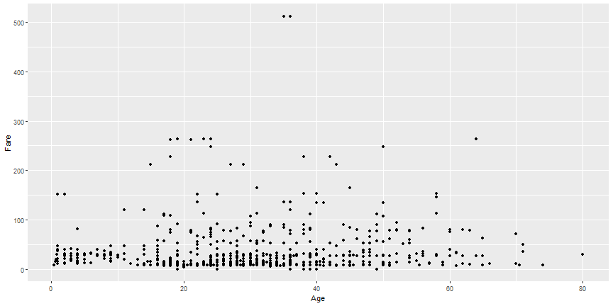
```

![](Figs/unnamed-chunk-63-1.png)
]

---
# Example

.pull-left[

Write the following function.  Give an example to test your function.

- Input: a data frame of two variables

- Output:

- a scatter plot of the two variables if both are continuous/numeric

- a bar chart of the two variables if none are continuous/numeric
  
  - print out 'This function cannot visualize your data' otherwise

]

.pull-right[
  
  - Test the function

```r
df$Pclass <- factor(df$Pclass)
d <- df %>% select(Sex, Pclass)
viz(d)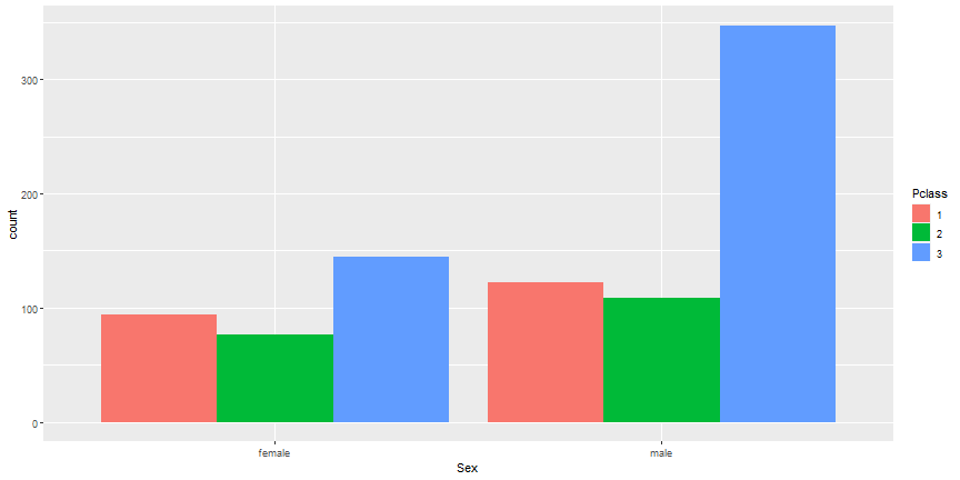
```

![](Figs/unnamed-chunk-64-1.png)
]

---
# Example

.pull-left[

Write the following function.  Give an example to test your function.

- Input: a data frame of two variables

- Output:

- a scatter plot of the two variables if both are continuous/numeric

- a bar chart of the two variables if none are continuous/numeric
  
  - print out 'This function cannot visualize your data' otherwise

]

.pull-right[
  
  - Test the function

```r
d <- df %>% select(Sex, Age)
viz(d)
```

```
## [1] "This function cannot visualize your data."
```
]

---
class: inverse, middle, center
# Optional

---
# Example

Write the following function.  Give an example to test your function.

- Input:

- input_data: a clean data frame with a variable name `target`. The `target` variable is also binary. 
  
  - train_percent: a number presenting a proportion of training data.

- Output: the plot of the decision model `rpart` where the training data is train_percent.

---
# Example

Write the following function.  Give an example to test your function.

- Input:

- input_data: a clean data frame with a variable name `target`. The `target` variable is also binary. 
  
  - train_percent: a number presenting a proportion of training data.

- Output: the plot of the decision model `rpart` where the training data is train_percent.

```r
modl <- function(input_data, train_percent)
{
library(caret)
set.seed(00000)
splitIndex <- createDataPartition(input_data$target, p = train_percent, 
                                  list = FALSE)
df_train <- input_data[ splitIndex,]
df_test <- input_data[-splitIndex,]
library(rpart)
tree1<-rpart(target ~ ., 
             data = df_train)
# Plot the tree
library(rattle)
fancyRpartPlot(tree1)
}
```

---
# Example - Test the function

```r
# Read in the data
df = read_csv("titanic.csv")

# Set the target variable
names(df)[8] <- 'target'

# Remove some columns
df$PassengerId =  NULL
df$Ticket =  NULL
df$Name = NULL
df$Cabin = NULL

# Correct variables' types
df$target <- factor(df$target)
df$Pclass = factor(df$Pclass)
df$Sex <- factor(df$Sex)
df$Embarked <- factor(df$Embarked)

# Handle missing values
df$Age[is.na(df$Age)] = mean(df$Age, na.rm = TRUE)

df = drop_na(df)
```

---
# Example - Test the function

```r
modl(input_data = df, train_percent = .7)
```

---
# Another way to call the function

```r
modl(df, .7)
```

---
# What if the user forgets an input

```r
modl(df)
```

---
# Set the default input

```r
modl2 <- function(input_data, train_percent = .7)
{
library(caret)
set.seed(00000)
splitIndex <- createDataPartition(input_data$target, p = train_percent, 
                                  list = FALSE)
df_train <- input_data[ splitIndex,]
df_test <- input_data[-splitIndex,]

library(rpart)
tree1<-rpart(target ~ ., 
             data = df_train)

# Plot the tree
library(rattle)
fancyRpartPlot(tree1)
}
```

---
# Example - Test the new function

```r
modl2(df)
```

---
# Example

Write the following function.  Give an example to test your function.

- Input:

- input_data: a clean data frame with a variable name `target`. The `target` variable is also binary. 
  
  - train_percent: a number presenting a proportion of training data. The default train_percent is .7

- Output: the accuracy of the random forest on test data trained by caret with `method = ranger`.  The proportion of the training data is p.

---
# Example

Write the following function.  Give an example to test your function.

- Input:

- Output: the accuracy of the random forest on test data trained by caret with `method = ranger`.  The proportion of the training data is p.

```r
modl3 <- function(input_data, train_percent=.7)
{
  library(caret)
set.seed(00000)
splitIndex <- createDataPartition(input_data$target, p = train_percent, 
                                  list = FALSE)
df_train <- input_data[ splitIndex,]
df_test <- input_data[-splitIndex,]
model <- train(target~., data=df_train, 
                        method = "ranger")
pred <- predict(model, df_test)
cm <- confusionMatrix(data = pred, reference = df_test$target)
cm$overall[1]
}
```

---
# Example - Test the function

```r
modl3(df)
```

```
##  Accuracy 
## 0.8496241
```